Introduction
When building calibration standards and kits, we were actively seeking test cases that would validate (or invalidate) the accuracy of the methods we develop. A straightforward test is measurement of an open-ended pigtail after calibration. The result is not an ideal open circuit, there is capacitance and actually radiation loss – unless one cuts the insulator and inner conductor extension along the outer conductor edge. But this is harsh verification, because the pigtail is destroyed upon doing so. Well, we’ve still done it many times and seen the open circuit response, but to bring in a new, independent validation test we came across an ingenious method introduced by Rohde&Schwarz in one of their application notes, the T-Check.
T-Check applies to 2-port measurements, and in nutshell it is based on a low-loss T-junction where the middle branch of the tee is terminated by a load ZL.
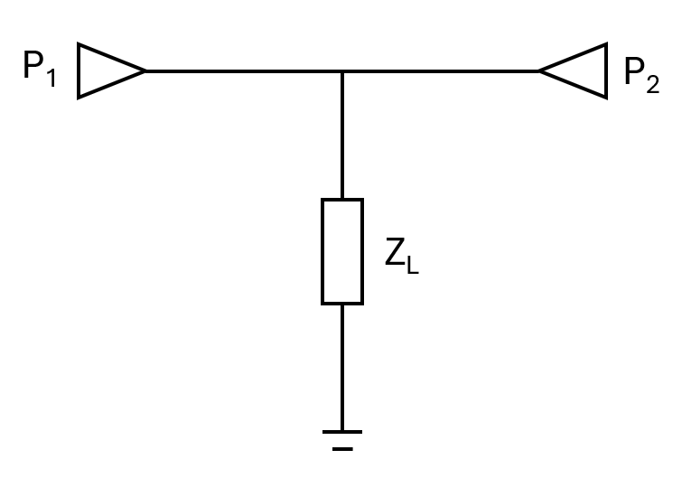
Figure 1: Basic principle of T-checker
The method makes use of the observation that under the assumption of a lossless tee, the product of |S13|·|S23| can be expressed by two formulas that are not mathematical identities (i.e. they cannot directly be derived from each other):

The ratio of (1):(2) is defined as the T-check parameter cT, and for a lossless system its value is exactly one.
The amazing beauty of T-check method is that theoretically cT does not depend on termination ZL, as long as it is not purely reactive. It can be for example 50 Ohms or 100 Ohms, and the parasitic reactances of a practical implementation do not matter – the cT is a very robust and tolerant parameter that basically depends only on the calibration and VNA quality. Moreover, the “specifications” for a T-Check hardware are so simple that one can easily build one, yet there are also commercial checkers. With any RF simulator or a simple script, one can readily evaluate formulas (1) and (2), and calculate the cT parameter.
Building a T-checker
With the intention to test Dicaliant pigtail calibration quality, we can’t utilize commercial T-checkers, because they are connectorized with SMA, as are the classical calibration kits. Nevertheless, it is easy to build a T-checker on PCB and connect pigtails on its ports.

Figure 2: T-checker built on PCB with ports connected to pigtails
Our T-checker is simply a short microstrip which has two 100 Ohm resistors in parallel. The dimensions are kept small (microstrip length = 2 mm) to obey the assumption of negligible losses as accurately as possible. For reference, we also built a T-checker using two SMA connectors face-to-face.

Figure 3: T-checker built from two SMA connectors. The load is connected between the inner conductor and the ground in the middle.
What if T-checker has losses?
A practical T-checker has always some losses. To estimate their impact, we simulated cT in scenarios that correspond to our physical T-checkers. Using QUCS Studio 4.3.1 package we built models for SMA- and PCB T-checkers with realistic metal and dielectric losses. The resulting cT curves up to 8.5 GHz are given in Figure 4.

Figure 4: Theoretical cT due to lossy T-checker
The result represents ideal VNA and ideal calibration, and we can see that the loss for these checkers accounts for 2-3% deviation from unity. The reference application note states that “Deviations of up to ±10% are considered as minor (green range). Deviations between 10% and 15% are still acceptable (yellow range) and those more than 15% should not occur in a good vector network analyzer after careful system error calibration.”
Because we can measure the T-checker losses before connecting the load – essentially using RHS of Eq. (2) – we can fit the loss model to measured losses and thus get a corrected ideal cT as a more accurate reference. Therefore, to simplify comparison, we adjust the measured cT accordingly to compensate the loss contribution, so that we can keep on using unity as the ideal result.
Results
The SMA T-checker result is straightforward – we used E-Cal automatic calibration kit for Pico VNA 108 and calculated cT from the resulting S-parameters, adjusting by the lossy ideal result. For the PCB T-checker, the same calibration for raw measurement was used, followed by de-embedding using 2-port pigtail model developed by Dicaliant. For comparison, we also applied classical port extension. The results are given in Fig. 5.
We can observe that, as expected, the conventional E-Cal calibration and Pico VNA 108 is doing a good job with the SMA T-checker. The deviation from ideal is less than 7% at all frequencies and less than 2% above 4 GHz.
The test for Dicaliant pigtail model performs also very well: the maximum deviation from ideal is less than 7% at all frequencies, and less than 5% above 4 GHz. Overall, the result conforms easily with the quantitative ±10% criterion of an accurate calibration.
In contrast, the port extension reaches the red alert region already at 2.4 GHz, and the safe range is limited up to 2 GHz.

Figure 5: Measured cT adjusted by lossy ideal model
Conclusions
The SMA T-checker method provides an elegant, unbribable validation of a 2-port VNA calibration accuracy. It is robust and simple enough to be built as a DIY device. The method can be used to detect frequency limits for reliable measurements, and specifically the Dicaliant de-embed model easily passes the test up to fmax=8.5 GHz. The classical port extension method fails the test above 2 GHz, aligning with previously accumulated evidence regarding the maximum valid frequency for this technique.
T-Check can also be used to monitor need for VNA factory recalibration. It may be a good idea to store the cT measurement now and then, and prepare for recalibration well before reaching the red region!